Euler Examples

Search

US Population Forecast

The data in this example are from an introductory example of Matlab.

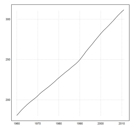
The following are numerical data of the US population in millions.

>p := [75.995, 91.972, 105.711, 123.203, 131.669, ...
      150.697, 179.323, 203.212, 226.505, 249.633, 281.422];
>t := 1900:10:2000;

Let us try to fit a polynomial to it the direct way. Since we do not want to get oscillation, we set the degree to 3.

>pf := polyfit(t,p,3); ...
 plot2d(t,p,points=true,a=1900,b=2010,c=0,d=320,yl="Millions"); ...
 plot2d("polyval(pf,x)",add=1):

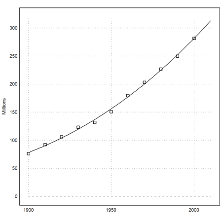
This does not look to bad. Let us evaluate the forecast for 2010.

>polyval(pf,2010)

312.691378788

For polynomials of higher degree, we get problems with overflows and inaccurate values. This can be avoided by re-scaling the date to [0,1].

Even then, the behavior of the polynomial gets erratic.

>pf1 := polyfit((t-1900)/50,p,10); ...
 plot2d(t,p,points=true,a=1900,b=2010,c=0,d=320); ...
 plot2d("polyval(pf1,(x-1900)/50)",add=1):

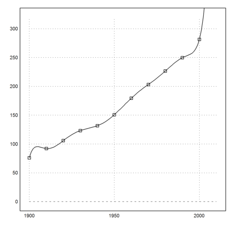
It is best to stay with polynomials of low degree. Or even better, to use a model, which is appropriate for population growth such as exponential models (see below).

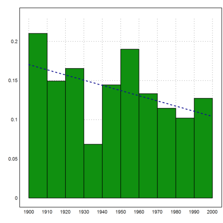
Let us have a look at the growth rate for each year.

>rate := differences(p)/(p[1:cols(p)-1])

[0.210238,  0.149382,  0.16547,  0.0687159,  0.144514,  0.189957,
0.133218,  0.114624,  0.102108,  0.127343]

>plot2d(t,rate,bar=true):

It looks decreasing with a problematic break at 1930-1940. We can try a linear fit.

>pr := polyfit(t[1:cols(t)-1],rate,1)

[1.42809,  -0.000661971]

>plot2d("polyval(pr,x)",color=blue,thickness=2,style="--",>add); insimg();

So we can predict the rate for the years 2000-2010.

>pc := polyval(pr,2000)

0.104148605987

If you look at the data, there is a trend to an increased production rate from 1990 to 2000. So we are sceptic, if such a long term prediction really applies.

However, we use it to predict the population in 2010.

>(1+pc)*p[-1]

310.731708994

The true number is 308 millions. It turns out the growth was a much less than predicted.

>(308-p[-1])/p[-1]

0.0944417991486

More recent Data

I found the following population data from 1960 to 2011 on

http://data.worldbank.org/country/united-states

To generate the file, I downloaded the Excel version and copied the line with the population data to a file. It contains a single tab separated line.

>t := 1960:2011; p := readmatrix("uspopulation.dat"); ...
 plot2d(t,p/1000000):

Let us try to determine the yearly growth rate from this.

>rate := differences(p)/head(p,-2); ...
 t1=head(t,-2); plot2d(t1,rate):

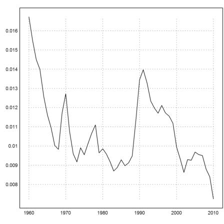
This looks quite erratic, but with a descending tendency. Note that sharp descent in the 1960-1968 due to the invention of the contraception.

Even, if we take only the data from 1990 on, it is obvious how dubious a long term prediction would be. Fitting some exponential curve to the data seems appropriate, but it is probably only like guessing.

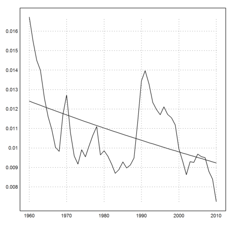
But we try to estimate the growth in 2011 using extrapolation.

>pr := polyfit(1990:2010,rate[-22:-2],1)

[0.501914,  -0.000245551]

>pc := polyval(pc,2011)

0.104148605987

Now we predict the number for 2012.

>p[-1], p[-1]*(1+pc), %-p[-1]

311591917
344043780.792
32451863.7924

The 2.5 million increase is in accordance with the data you will find in the net.

By the way, the 10 year rate based on the same rate per year would be the following.

>(1+polyval(pc,2011))^10-1

1.69324141904

This is much less than the 9.4% we predicted with the data in the last section.

Fitting an Exponential Model

The following code can be used to fit an exponential model to the reproduction rate.

>function expmodel (x,p) := p[1]*exp(p[2]*(x-1960)); ...
 t1=head(t,-2); topt=modelfit("expmodel",[0.01,-0.1],t1,rate)

[0.0124051,  -0.00589948]

However, the result is not very satisfying due to the erratic and unpredictable changes in the past.

>plot2d(t1,rate); plot2d(t1,expmodel(t1,topt),>add):

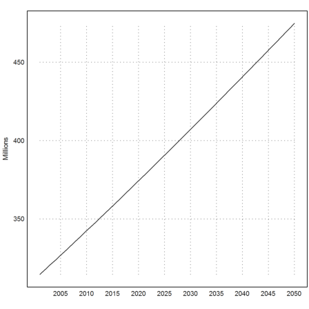
Assuming this prediction model of the growth rate, we can predict the grows rate for each year until 2050. Then we can predict the development of the US population.

Weather or not this has anything to do with reality is an open question.

>t2=2001:2050; rate2=expmodel(t2,popt);  ...
 plot2d(t2,cumprod(1+rate2)*p[-1]/1000000,yl="Millions"):

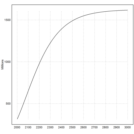
Just for the sake of our study we remark that the population converges to a value with our exponential model.

>t2=2001:3000; rate2=expmodel(t2,popt);  ...
 plot2d(t2,cumprod(1+rate2)*p[-1]/1000000,yl="Millions"):

Examples